Fit A Model (Levenberg-Marquardt Method)
The Fit A Model (Levenberg-Marquardt Method) command fits a data set to an equivalent-circuit model stored on your computer’s disk. The model can be one of the standard models supplied with the EIS software, or it can be a custom model you generated via the model editor.
The EIS system uses a complex, non-linear c² minimization to fit the impedance data to the selected equivalent-circuit model. Each model includes a number of adjustable parameters. Examples of adjustable parameters include:
- The cell’s uncompensated resistance.
- The cell’s double-layer capacitance.
- The pore resistance of a sample with a defective paint coating.
The fitting routine searches for the parameter values that cause the model’s impedance spectrum to most closely match the experimental spectrum.
The minimization algorithm is quite complex. It makes a number of estimates for the values of the adjustable parameters. After each estimate, a “goodness of fit” is evaluated. New estimates for the parameter values are then made, using the well-known Levenburg-Marquardt algorithm. The process is repeated until the fit stops improving, or until a preset number of iterations have been made.
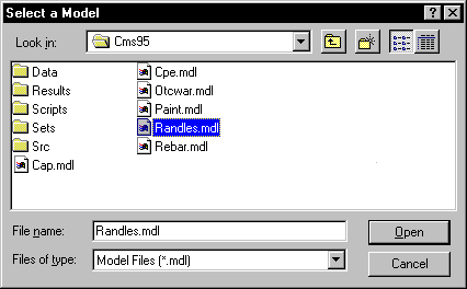
Below is the Select a Model dialog box that appears when you select the Fit A Model (Levenberg-Marquardt Method) command. Models are stored with a filename extension of .MDL. Generating equivalent-circuit models is described in the next section.

- Click here for a description of the standard equivalent-circuit models provided with the EIS software.
- Click here for a list of the adjustable parameters for each of the standard models.
After you choose a model, the system displays a Parameter Initialization dialog box. Each of the adjustable parameters in the model is listed on a separate line in this dialog box. The first field on each parameter line is the initial estimate that the fit will use for the parameter. This initial parameter is set in the model file, and can be changed in the model editor. After the first fit, the values of the parameters are set to the last entered values or the last calculated values. To set these values back to default, click the Reset to Default Values button.
Do not click the Calculate button until you have non-zero values for all the initial parameter estimates. Initial parameter values that are close to the fit values speed the fitting process and minimize non-convergence problems.
If you know the value of one of the model’s adjustable parameters exactly, enter the known value in the parameter’s field and activate the Lock checkbox for that parameter. The fitter does not vary a parameter with an active Lock checkbox.
The Iterations field allows you to control the maximum number of iterations (optimization loops). The fitting process is repeated until the fit stops improving, or until the maximum number of iterations has been made. If the fit does not converge on a first attempt, increase the number in the Iterations field and try again.
Control buttons in the Parameter Initialization dialog box
Close button
- Concludes the curve-fitting and writes the current values of the parameters to the New Page.
Preview button
- Calculates the impedance spectrum of the model using the initial values for all the adjustable parameters. Plots this model spectrum on the same chart as your data curve.
- This command is useful when you are interested in manually changing values and previewing the corresponding fit.
Calculate button
- Begins the curve-fitting procedure using the initial values displayed. You can click this button repeatedly to achieve a better fit by running more iterations.
Reset to Default Values button
- Resets all of the parameter values to the initial values stored in the model.
The time required to fit a spectrum to a model depends on the speed of your computer, the number of parameters in the model, the number of points in the spectrum, and the degree to which the model describes the spectrum. In most cases the fit should finish within a few seconds.
NOTE: There will be some cases in which the fit does not converge to a reasonable set of values. This situation can be detected quite easily on the graph: The fit plotted on the chart does not even remotely resemble the original data.
Several factors can cause a convergence failure:
- Fitting to an incorrect model. This is the most common problem. Increasing the number of iterations or improving the initial estimates cannot help the least-squares algorithm fit an incorrect model to a data set. Try a different model.
- Not enough iterations. Try increasing the value of the Iterations parameter in the Parameter Initialization dialog box.
- Poor initial estimates for one or more of the fit parameters. Try different values.
- Stray data points in the data set. Disable any stray data points by right-clicking on the point and selecting Disable. Alternatively, the fit is performed on the selected region (or the full data set if no region is selected). You can select a smaller region for your data set. If a data point is disabled, it will not be used, even if in the selected region. To re-enable a point, right -lick on the point and choose Enable. To disable or enable multiple points, select those points with the Select Portion of Curve tool
 , and then right-click on any point to specify Disable or Enable.
After the fit is finished, the script
- Calculates the impedance spectrum of the model using the fit values for the adjustable parameters.
- Plots this model spectrum on the same chart as your data curve. This includes both the Bode and Nyquist charts.
- Upon closing the Model Parameter window, the impedance analysis script generates a list of the fit values and the estimated errors for the fit values. This list is written to a new page which has the same name as the model.

Comments are closed.