Quantitative Corrosion Theory

In Electrochemical Basis of Corrosion, we pointed out that Icorr cannot be measured directly. In many cases you can estimate it from current-versus-voltage data. You can plot a logarithmic current-versus-potential curve over a range of about one half volt. The voltage scan is centered on Eoc. You then fit the measured data to a theoretical model of the corrosion process.

The model we use assumes that the rates of both the anodic and cathodic processes are controlled by the kinetics of the electron-transfer reaction at the metal surface. This is generally true for corrosion reactions. An electrochemical reaction under kinetic control obeys the following equation, the Tafel equation.

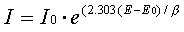
In this equation,

I is the current resulting from the reaction,

I0 is a reaction-dependent constant called the exchange current,

E is the electrode potential,

E0 is the equilibrium potential (constant for a given reaction),

β is the reaction’s Beta coefficient (constant for a given reaction); β has units of volts/decade.

The Tafel equation describes the behavior of one isolated reaction. But in a corrosion system, we have two opposing reactions.

The Tafel equations for both the anodic and cathodic reactions in a corrosion system can be combined to generate the Butler-Volmer equation seen below.

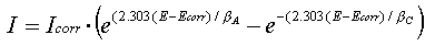
where

I is the measured cell current in amps,

Icorr is the corrosion current in amps,

Ecorr is the corrosion potential in volts,

βA is the anodic beta (Tafel) coefficient in volts/decade,

βC is the cathodic beta (Tafel) coefficient in volts/decade.

What does the Butler-Volmer equation predict about the current-versus-voltage curve? At Ecorr each exponential term equals one. The cell current is therefore zero, as you would expect. Near Ecorr, both exponential terms contribute to the overall current. Finally, as you get far from Ecorr, one exponential term predominates and the other term can be ignored. When this occurs, a plot of log(current) versus potential becomes a straight line.

A log I versus E plot is generally called a Tafel plot.

In practice many corrosion systems are kinetically controlled and thus obey the Butler-Volmer Equation. A log(current)-versus-potential curve that is linear on both sides of Ecorr is indicative of kinetic control for the system being studied. However, there can be complications, such as:

• Concentration polarization, where the rate of a reaction is controlled by the rate at which reactants arrive at the metal surface. Often cathodic reactions show concentration polarization at higher currents, when diffusion of oxygen or hydrogen ion is not fast enough to sustain the kinetically controlled rate.
• Oxide formation, which may lead to passivation, can alter the surface of the sample being tested. The original surface and the altered surface may have different values for the constants in the Butler-Volmer equation.
• Other effects that alter the surface, such as preferential dissolution of one component of an alloy, can also cause problems.
• A mixed control process, where more than one cathodic or anodic reaction occurs simultaneously, complicates the model. An example of mixed control is the simultaneous reduction of oxygen and hydrogen ion.
• Finally, potential drop as a result of cell current flowing through the resistance of your cell solution causes errors in the kinetic model. This last effect, if it is not too severe, may be correctable via IR-compensation in the potentiostat.

In most cases, complications like those listed above cause non-linearities in the Tafel plot. Use with caution the numbers that arise from a Tafel analysis on data that do not have a linear Tafel plot.

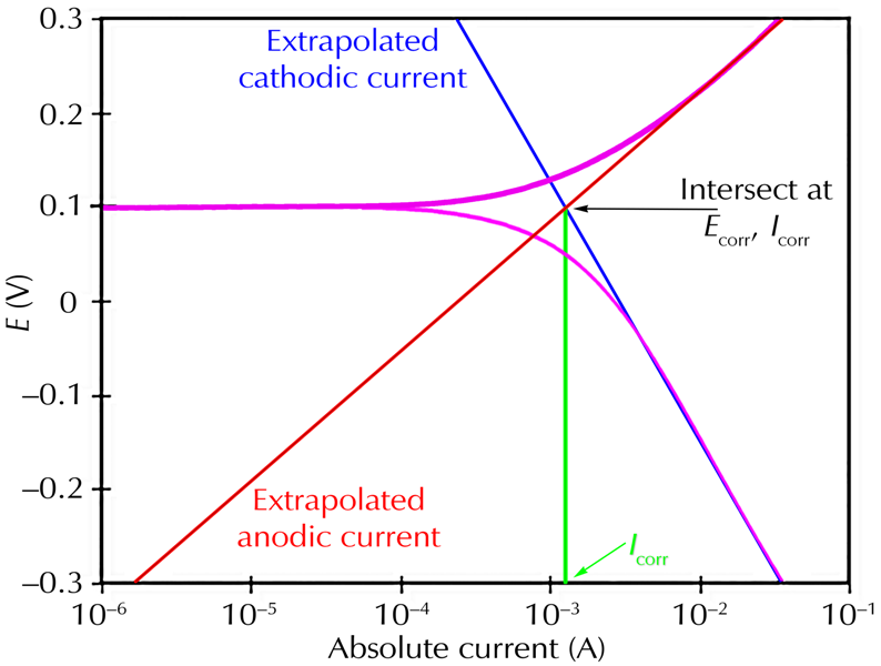
Classic Tafel analysis is performed by extrapolating the linear portions of a log(current)-versus-potential plot back to their intersection. See the figure below. The value of either current at the intersection is Icorr. Unfortunately, many real-world corrosion systems do not provide a sufficient linear region to permit accurate extrapolation. Most modern corrosion-test software performs a more sophisticated numerical fit to the Butler-Volmer equation. The measured data is fit to the Butler Volmer equation by adjusting the values of Ecorr, Icorr, βA, and βC. The curve-fitting method has the advantage that it does not require a fully-developed linear portion of the curve.

Classic Tafel Analysis

You can further simplify the Butler Volmer equation by restricting the potential to be very near to Ecorr. Close to Ecorr, the current-versus-voltage curve approximates a straight line. The slope of this line has the units of resistance (Ω). The slope is called the Polarization Resistance, Rp. An Rp value can be combined with an estimate of the β coefficients to yield an estimate of the corrosion current.

If we approximate the exponential terms in the Butler-Volmer equation with the first two terms of a power-series expansion (ex = 1 + x + x2/2…) and simplify, we get one form of the Stern-Geary equation:

Icorr = (1/ Rp) (βAβC / 2.303 (βA + βC) )

In a Polarization Resistance experiment you record a current-versus-voltage curve as the cell voltage is swept over a small range near Eoc. A numerical fit of the curve yields a value for the Rp. Polarization Resistance data does not provide any information about the values for the β coefficients. Therefore, to use the Stern-Geary equation, you must provide β values. These can be obtained from separate Tafel-type experiments or estimated from your experience with the system you are testing.