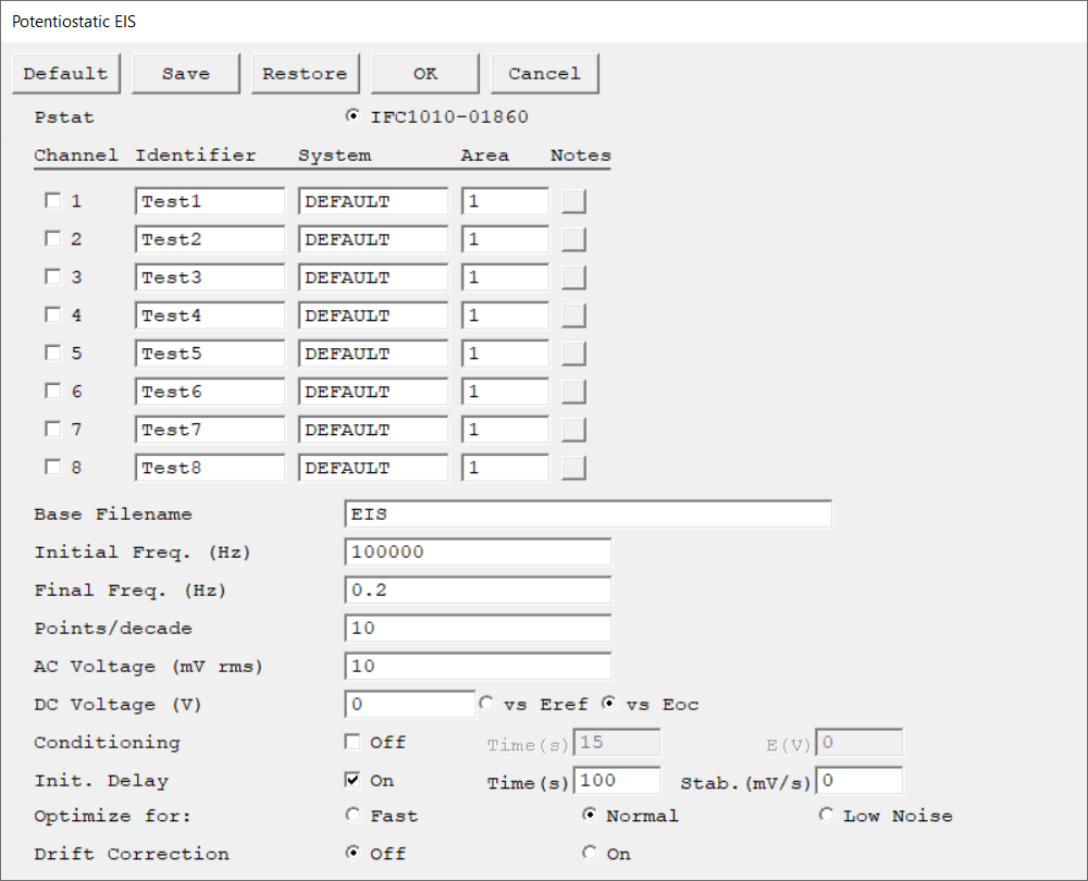
Select the potentiostat/galvanostat to perform the experiment. Each radio button corresponds to an installed potentiostat. You can select only one potentiostat at a time. Potentiostats that are already in use are marked with an asterisk. They can be selected but cannot be used.
Channel
There is one Channel Setup switch for each of the 8 channels. Click the checkbox to select a specific channel. As the script loops through the channels, it only runs tests on channels that are selected. The selected channel numbers do not have to be continuous.
Identifier
A string that is used as a name. It is written to the data file, so it can be used to identify the data in database or data manipulation programs.
The ChannelIdentifier string is virtually identical to the Test Identifier string. The only difference is that in multiplexed tests, the Identifier refers to an experiment run on a single cell and not to the entire experimental run.
System
Select a set of electrochemical parameters relevant to your particular test system. The parameters are recovered from the system parameter database file. The recovered parameters are all used for the calculation of the corrosion rate. They are the sample's equivalent weight, density, anodic β and cathodic β. When you attempt to run an experiment, the system searches the SYSTEM.SET file for a parameter set stored under the name in the System parameter. If the software finds no parameter set, an error message appears and you are returned to the Setup dialog box.
Area
The electrode area that is used in calculations. It can be set individually for each channel.
cm2
Notes
Enter several lines of text that describe the experiment. There is a separate entry for each channel in a multiplexed test. A typical use of Channel Notes is to record the experimental conditions for a data set.
The Channel Notes controls are similar to the Notes control described for non-multiplexed experiments.
Base Filename
Each channel has its own data file. The Base Filename is used to derive the filenames for these files. The filename for ChannelN (1–8) is created by appending the character N to the Base Filename, then adding a *.DTA filename extension.
If the Base Filename is MYMUXDATA, the data file for Channel 1 is named MYMUXDATA1.DTA. The filename resulting from the concatenation of the Base Filename and the channel number must adhere to Windows® filename conventions. Avoid punctuation characters (the underscore, "_", is OK). You are allowed a maximum of 250 (not 255) characters in the Base Filename. The extra characters are reserved for the channel number appended to the Base Filename. Do not include *.DTA when specifying the Base Filename. It is automatically added when the full data file name is generated.
Initial Freq.
The starting frequency of the frequency sweep during data acquisition.
EIS scans are usually run with the Initial Freq. larger than the Final Freq. parameter. Refer to the potentiostat's Operator's Manual for detailed information on the applicable frequency range.
hertz (Hz)
Final Freq.
The final frequency of the frequency sweep during data acquisition.
The frequency sweep may not stop exactly at the final frequency. It is mathematically impossible to control both Points/decade and Final Freq. parameters exactly for all scan ranges. The EIS software chooses to control the Points/decade parameter exactly.
hertz (Hz)
Points/decade
The data density of the measured impedance spectrum. The data are spaced logarithmically and the number of data points in each frequency decade equals Points/decade. As a consequence, the frequency sweep may not stop exactly at the final frequency. It is guaranteed to do so only when the scan range contains an integer number of decades, such as 5 kHz to 0.05 Hz (five decades). You can use Initial Freq., Final Freq., and Points/decade to calculate the total number of data points in the spectrum.
Assuming that Initial Freq. = 5000 Hz, Final Freq. = 0.2 Hz, and Points/decade = 10:
The estimated number of points is always converted to an integer by truncating the fractional part of the number. The spectrum cannot contain more than 32000 data points. This is not a critical limitation because most impedance spectra contain fewer than 100 points.
AC Voltage
The amplitude of the AC Voltage signal applied to the cell. Multiply the entered root-mean-square (rms) value by √2 (or ~1.414) to convert into a peak value.
Generally, you can enter AC Voltage values between 0.1 mV and 3000 mV. Values greater than 25 mV cause a non-linear response in most electrochemical systems and are therefore not recommended. The system does not control the AC Voltage exactly. It is satisfied with an AC Voltage close to the desired value. However, this inaccuracy does not carry over into the measured impedance, because an accurately measured AC Voltage is used in the impedance calculation.
Generally, you can enter AC Voltage values between 1 mV and 1000 mV. The system does not control the AC Voltage exactly. At higher frequencies, the potentiostat often cannot maintain a one-to-one ratio between the AC signal at the potentiostat input and the resulting signal between the working and reference electrodes. The input signal may need to be 10 or even 100 times larger than the output signal. The EIS system automatically compensates for this effect. When it does so, it adjusts the applied signal such that the measured AC potential is close to being correct. It does not attempt to keep the measured E signal exactly equal to the AC Voltage parameter. In some cases, the potentiostat simply cannot apply the requested AC voltage. This occurs at high frequency on cells with high solution-resistance. An error message such asUnable to Control AC Cell Voltage should appear on the real-time display. If you see this message, try lowering your frequency, lowering the setting on the AC Voltage parameter, or lowering your cell's solution resistance.
mV rms
DC Voltage
The constant potential applied to the cell throughout the frequency sweep. The AC Voltage is summed with the DC Voltage. The allowed range is ±8 V with a resolution of 0.125 mV. The voltage can be entered relative to the reference electrode potential (vs. Eref) or relative to the open-circuit potential (vs. Eoc). If the DC Voltage is entered vs. Eoc, the sum of the measured Eoc and the entered DC Voltage must be within the range of ± 8 V.
volts (V)
Conditioning
You may condition the electrode as the first step of the experiment, e.g., to remove an oxide film from the electrode or to grow one. Conditioning ensures that the metal sample has a known surface state at the start of the experiment. This step is done potentiostatically for a set amount of time.
Turn the conditioning phase On or Off with the Conditioning switch check box. Conditioning E is the potential applied during the conditioning phase of the experimental sequence. The conditioning potential has an allowed range of ±8 V. The resolution is 0.25 mV. If you have iR-compensation enabled for the data acquisition phase of your experiment, it is also turned on during conditioning. Conditioning E is always specified vs. Eref, because the open-circuit potential is not measured until after Conditioning is completed.
The Conditioning Time is the length of time that the sample is potentiostatted at Conditioning E. The minimum time is 1 s and the maximum time is 400000 s (more than 4 days). Below 1000 seconds, the time resolution is 1 s. Between 1000 and 10000 seconds, the resolution is 10 s, and 100 s above 10000 seconds.
seconds (s), volts (V)
Init. Delay
The Initial Delay phase of the experiment is the first step to occur in the experimental sequence. This phase of the experiment stabilizes the open-circuit potential of the sample prior to any applied signal and measures that open-circuit potential.
The Initial Delay is turned On or Off via the check box in the Setup dialog. The Initial Delay Time parameter is the time that the sample is held at the open-circuit potential prior to the scan. The delay may stop before the Initial Delay Time if the Stability criterion for Eoc is met. The minimum Delay Time time is 1 s and the maximum time is 400000 s (more than 4 days). Below 1000 seconds, the time resolution is 1 s. Between 1000 and 10000 seconds, the resolution is 10 s, and 100 s above 10000 seconds.
In many cases, you really do not want to set a delay for a fixed time, but you may want to a delay until Eoc stops drifting. The Stability parameter allows you to set a drift-rate that you feel represents a stable Eoc. If the absolute value of the drift-rate falls below the Stability parameter, the Initial Delay phase of the experiment ends immediately, disregarding the programmed Initial Delay Time. Enter a Stability setting of zero to ensure that the delay will last for the full Initial Delay Time. A typical value is 0.05 mV/s. The upper limit of this parameter is 8 V/s, well above the range of practical stabilities with real cells, while the lower limit is set by your patience. A stability of 0.01 mV/s indicates a drift of less than 1 mV within 100 seconds. The software will always take data long enough to resolve a 1 mV change in the potential at the requested drift rate.
No open-circuit voltage measurement occurs if the initial delay is turned off. In this case, the open-circuit voltage defaults to 0.0 V.
seconds (s), mV/s
Optimize for
Select the sampling method for the experiment:
•Fast is the appropriate selection when the cell's stability is poor and a spectrum must be measured rapidly, or the system's impedance is low and well defined.
•Normal is the appropriate selection when the cell's impedance is high or the electrochemical system is noisy.
•The best data can be taken with Low Noise, but the time required to record an EIS spectrum can be quite long.
The EIS system tries to explain 99.9% of the variation in each Lissajous curve by fitting the E and I data to sine waves at the excitation frequency. It will record and average as many as 20 Lissajous curves to achieve this accuracy. There is a two-second delay after each data point to allow you to examine a Bode plot of the impedance spectrum.
With Fast, the time required to record a spectrum is much shorter (often by a factor of five). The fit accuracy is reduced from 99.9% to 99.5%. The maximum number of Lissajous curves is reduced, as low as two at low frequencies. The Lissajous curve is not displayed after the first ranging point, so there is no need for delays when the display changes.
Drift Correction
Select On to enable Drift Correction. Both the original and the drift-corrected impedance values are separately calculated and recorded. The drift corrected impedance plot will be active by default but can be changed from the drop-down menu above the chart.
Drift Correction fits current and voltage data to a sine wave using a linear drift term, followed by non-linear least squares regression. Drift data are then subtracted from the current and voltage values and the corrected impedance Z is calculated via Fourier analysis.
Drift Correction is always disabled if an overload is detected, the frequency is above 10 Hz, or cycle decimation is occurring. Drift most commonly occurs at lower frequencies, which is why limitations are applied to this frequency range.