Description
Parameter |
Description |
Units |
||
|---|---|---|---|---|
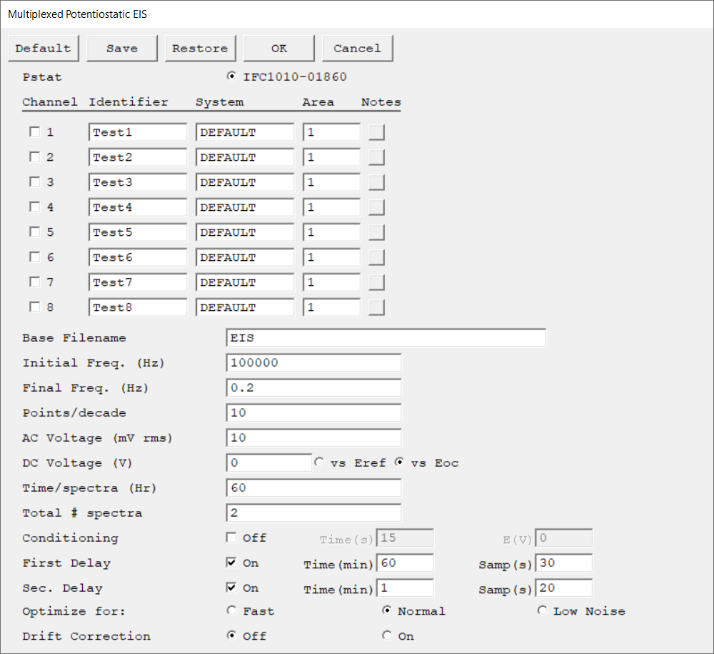
Select the potentiostat/galvanostat to perform the experiment. Each radio button corresponds to an installed potentiostat. You can select only one potentiostat at a time. Potentiostats that are already in use are marked with an asterisk. They can be selected but cannot be used.
|
|
|||
There is one Channel Setup switch for each of the 8 channels. Click the checkbox to select a specific channel. As the script loops through the channels, it only runs tests on channels that are selected. The selected channel numbers do not have to be continuous. |
|
|||
A string that is used as a name. It is written to the data file, so it can be used to identify the data in database or data manipulation programs.
The Channel Identifier string is virtually identical to the Test Identifier string. The only difference is that in multiplexed tests, the Identifier refers to an experiment run on a single cell and not to the entire experimental run. |
|
|||
Select a set of electrochemical parameters relevant to your particular test system. The parameters are recovered from the system parameter database file. The recovered parameters are all used for the calculation of the corrosion rate. They are the sample's equivalent weight, density, anodic β and cathodic β. When you attempt to run an experiment, the system searches the SYSTEM.SET file for a parameter set stored under the name in the System parameter. If the software finds no parameter set, an error message appears and you are returned to the Setup dialog box. |
|
|||
The electrode area that is used in calculations. It can be set individually for each channel. |
cm2 |
|||
Enter several lines of text that describe the experiment. There is a separate entry for each channel in a multiplexed test. A typical use of Channel Notes is to record the experimental conditions for a data set.
The Channel Notes controls are similar to the Notes control described for non-multiplexed experiments. |
|
|||
Each channel has its own data file. The Base Filename is used to derive the filenames for these files. The filename for Channel N (1–8) is created by appending the character N to the Base Filename, then adding a *.DTA filename extension.
|
|
|||
The starting frequency of the frequency sweep during data acquisition.
|
hertz (Hz) |
|||
The final frequency of the frequency sweep during data acquisition.
|
hertz (Hz) |
|||
The data density of the measured impedance spectrum. The data are spaced logarithmically and the number of data points in each frequency decade equals Points/decade. As a consequence, the frequency sweep may not stop exactly at the final frequency. It is guaranteed to do so only when the scan range contains an integer number of decades, such as 5 kHz to 0.05 Hz (five decades). You can use Initial Freq., Final Freq., and Points/decade to calculate the total number of data points in the spectrum.
|
|
|||
The amplitude of the AC Voltage signal applied to the cell. Multiply the entered root-mean-square (rms) value by √2 (or ~1.414) to convert into a peak value.
|
mV rms |
|||
The constant potential applied to the cell throughout the frequency sweep. The AC Voltage is summed with the DC Voltage. The allowed range is ±8 V with a resolution of 0.125 mV. The voltage can be entered relative to the reference electrode potential (vs. Eref) or relative to the open-circuit potential (vs. Eoc). If the DC Voltage is entered vs. Eoc, the sum of the measured Eoc and the entered DC Voltage must be within the range of ± 8 V. |
volts (V) |
|||
The time interval between the start of each spectrum. The Time/spectra parameter must be set to a time longer than the time required to acquire each spectrum.
|
hours (hr) |
|||
The number of spectra generated in the test. If you want EIS data for 24 hours at 0.20 hours per spectrum, you should enter 120 as the Total # spectra parameter. |
|
|||
You may condition the electrode as the first step of the experiment, e.g., to remove an oxide film from the electrode or to grow one. Conditioning ensures that the metal sample has a known surface state at the start of the experiment. This step is done potentiostatically for a set amount of time.
|
seconds (s), volts (V) |
|||
Use the First Delay parameter to tell the system your definition of a stable potential and when to begin the actual measurement before the first spectrum is acquired.
If the absolute value of the stability criterion (Stab.) exceeds the set value, the First Delay phase ends immediately, disregarding the Time parameter, and the experiment begins. For example, a stability of 0.01 mV/s indicates a drift of less than 1 mV within 100 seconds. |
minutes (min), seconds (s) |
|||
Use the Secondary Delay parameter to tell the system your definition of a stable potential and when to begin the actual measurement after the first spectrum is acquired.
If the absolute value of the stability criterion (Stab.) exceeds the set parameter, the Sec. Delay phase ends immediately, disregarding the Time parameter, and the experiment begins. For example, a stability of 0.01 mV/s indicates a drift of less than 1 mV within 100 seconds. |
minutes (min), seconds (s) |
|||
Select the sampling method for the experiment: •Fast is the appropriate selection when the cell's stability is poor and a spectrum must be measured rapidly, or the system's impedance is low and well defined. •Normal is the appropriate selection when the cell's impedance is high or the electrochemical system is noisy. •The best data can be taken with Low Noise, but the time required to record an EIS spectrum can be quite long.
|
|
|||
Select On to enable Drift Correction. Both the original and the drift-corrected impedance values are separately calculated and recorded. The drift corrected impedance plot will be active by default but can be changed from the drop-down menu above the chart.
Drift Correction fits current and voltage data to a sine wave using a linear drift term, followed by non-linear least squares regression. Drift data are then subtracted from the current and voltage values and the corrected impedance Z is calculated via Fourier analysis.
|
|

