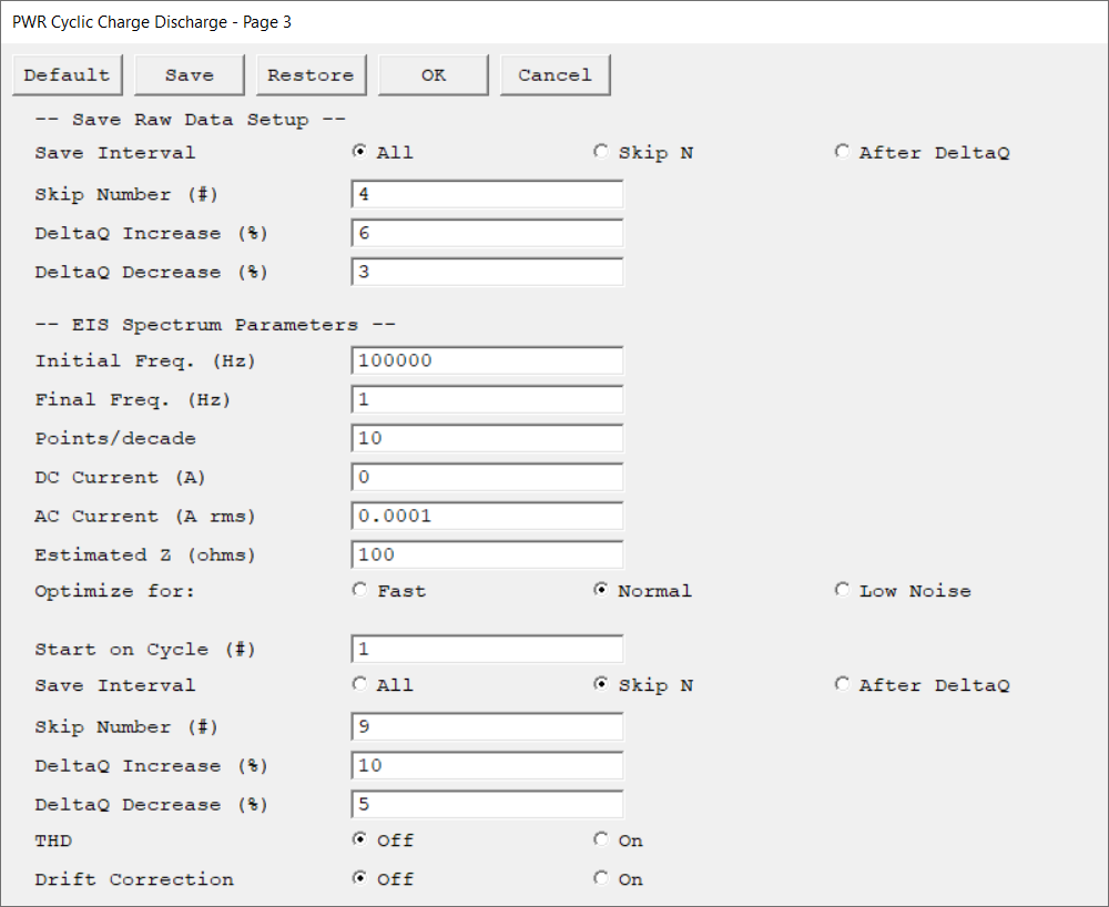
Set the interval for which Raw Data files are saved:
•All: Save all data files.
•Skip N: Save every (N + 1) cycle, skipping over Skip NumberN data points. For example, N = 4 saves every fifth data point.
•After Delta Q: Save data after a certain percentage change in charge Q specified in Delta Q Increase and Delta Q Decrease.
Skip Number
Specify the frequency at which raw data files are saved. If this number is zero, files are saved for every charge-discharge cycle. If the Skip # is set to a value greater than zero, n cycles are skipped for each cycle that is saved.
For example, if Skip # is set to 4, the 1st cycle is saved, the next four cycles (2, 3, 4, and 5) are skipped, cycle 6 is saved, cycles 7, 8, 9, and 10 are skipped, cycle 11 is saved, and so on.
Delta Q Increase
The percentage change in charge Q which must occur before the system starts recording raw data points, if you have selected Yes to Save Raw Data.
percent (%)
Delta Q Decrease
Initial Freq.
The starting frequency of the frequency sweep during data acquisition.
EIS scans are usually run with the Initial Freq. larger than the Final Freq. parameter. Refer to the potentiostat's Operator's Manual for detailed information on the applicable frequency range.
hertz (Hz)
Final Freq.
The final frequency of the frequency sweep during data acquisition.
The frequency sweep may not stop exactly at the final frequency. It is mathematically impossible to control both Points/decade and Final Freq. parameters exactly for all scan ranges. The EIS software chooses to control the Points/decade parameter exactly.
hertz (Hz)
Points/decade
The data density of the measured impedance spectrum. The data are spaced logarithmically and the number of data points in each frequency decade equals Points/decade. As a consequence, the frequency sweep may not stop exactly at the final frequency. It is guaranteed to do so only when the scan range contains an integer number of decades, such as 5 kHz to 0.05 Hz (five decades). You can use Initial Freq., Final Freq., and Points/decade to calculate the total number of data points in the spectrum.
Assuming that Initial Freq. = 5000 Hz, Final Freq. = 0.2 Hz, and Points/decade = 10:
The estimated number of points is always converted to an integer by truncating the fractional part of the number. The spectrum cannot contain more than 32000 data points. This is not a critical limitation because most impedance spectra contain fewer than 100 points.
DC Current
The constant current applied to the cell throughout the frequency sweep. The AC Current is summed with the DC Current. In most cases, the DC Current should remain at its default value of zero. The discussion of the AC Current describes some limitations on the DC Current value.
amperes (A)
AC Current
The amplitude of the AC signal applied to the cell. Multiply the entered root-mean-square (rms) value by √2 (or ~1.414) to convert into a peak value.
To convert the entered root-mean-square (rms) value into a peak-to-peak value, multiply by 2√2 (or ~2.83).
The range of the AC Current parameter is a complex topic. You want an AC Current that keeps the electrochemical cell in a pseudo-linear region of its current-to-voltage curve. In general, avoid AC Currents that create an rms-voltage larger than 25 mV. If your DC Current is zero, the largest AC Current you should enter is about 60% of the instrument's maximum compliance current. You cannot enter the full compliance current, because you are specifying an rms-value that is smaller than the peak value.
If your DC Current is not zero, you must make sure that the sum of the absolute value of the DC Current and 1.414 times the AC Current does not exceed the instrument's compliance current. If your DC Current is zero, the smallest AC Current that you should enter is a function of the maximum frequency in your experiment. Calculate the ratio of your maximum frequency divided by 100 kHz. Do not enter a current smaller than 5 mA times this ratio. For example, if your maximum frequency is 1 kHz, you can enter a current as small as 50 nA. Regardless of the frequency, we do not recommend entering an AC Current less than 1 nA. If you have a non-zero DC current, we recommend that your AC Current be within two orders of magnitude of the DC Current (between 1% of the DC Current and 100 times the DC Current).
The system does not control the AC Current exactly. At higher frequencies, the potentiostat often cannot maintain a one-to-one ratio between the AC signal at the galvanostat input and the resulting current signal. The EIS system automatically compensates for this effect. To do so, it adjusts the applied signal such that the measured AC current is close to being correct. It does not attempt to keep the measured I signal exactly equal to the AC Current parameter. The measured impedance relies on a measured AC Current so this lack of accuracy does to carry over to the experimental results. In some cases, the potentiostat simply cannot apply the requested AC Current. This occurs at high frequency on cells with high solution-resistance. An error message such as Unable to Control AC Cell Current should appear on the real-time display. If you see this message, try limiting your sweep range to avoid higher frequencies, lowering the setting on the AC Current parameter, or lowering your cell's solution resistance.
amperes (A) rms
Estimated Z
A user-entered estimate of the cell's impedance at the Initial Freq. parameter. It is used to limit the number of trials required before acquiring the first data point in an impedance spectrum. It is generally sufficient if Estimated Z is within a factor of five of the cell's impedance.
Before taking the first data point, the EIS software sets up the potentiostat and frequency response analyzer (FRA) to measure an impedance equal to Estimated Z and tries to measure the cell's impedance. If the estimate is fairly accurate, the first (or second) attempt to measure the impedance succeeds. If the estimate is poor, the system may take up to five trial readings before it finds the correct settings:
•After the first data point, the last measured impedance is used to calculate new measurement settings, so the entered Estimated Z becomes unimportant.
•An accurate Estimated Z is more valuable when the initial frequency is low. Remember, 1 mHz is 1000 s per cycle. Each impedance reading requires at least three cycles at a given frequency, so five readings to find a range at 1 mHz will take over 4 hours!
•There is no reason to enter values larger than 1 TΩ (1012Ω or smaller than 0.01 Ω, because these values drive the system settings to their most sensitive and least sensitive settings, respectively.After the first data point, the last measured impedance is used to calculate new measurement settings, so the entered Estimated Z becomes unimportant.
ohm
Optimize for
Select the sampling method for the experiment:
•Fast is the appropriate selection when the cell's stability is poor and a spectrum must be measured rapidly, or the system's impedance is low and well defined.
•Normal is the appropriate selection when the cell's impedance is high or the electrochemical system is noisy.
•The best data can be taken with Low Noise, but the time required to record an EIS spectrum can be quite long.
The EIS system tries to explain 99.9% of the variation in each Lissajous curve by fitting the E and I data to sine waves at the excitation frequency. It will record and average as many as 20 Lissajous curves to achieve this accuracy. There is a two-second delay after each data point to allow you to examine a Bode plot of the impedance spectrum.
With Fast, the time required to record a spectrum is much shorter (often by a factor of five). The fit accuracy is reduced from 99.9% to 99.5%. The maximum number of Lissajous curves is reduced, as low as two at low frequencies. The Lissajous curve is not displayed after the first ranging point, so there is no need for delays when the display changes.
Start on Cycle
Set the cycle number of the first EIS measurement.
Save Interval
Set the interval for which Raw Data files are saved:
•All: Save all data files.
•Skip N: Save every (N + 1) cycle, skipping over Skip NumberN data points. For example, N = 4 saves every fifth data point.
•After Delta Q: Save data after a certain percentage change in charge Q specified in Delta Q Increase and Delta Q Decrease.
Skip Number
Specify the frequency at which raw data files are saved. If this number is zero, files are saved for every charge-discharge cycle. If the Skip # is set to a value greater than zero, n cycles are skipped for each cycle that is saved.
For example, if Skip # is set to 4, the 1st cycle is saved, the next four cycles (2, 3, 4, and 5) are skipped, cycle 6 is saved, cycles 7, 8, 9, and 10 are skipped, cycle 11 is saved, and so on.
Delta Q Increase
The percentage change in charge Q which must occur before the system starts recording raw data points, if you have selected Yes to Save Raw Data.
percent (%)
Delta Q Decrease
THD
Enable Total Harmonic Distortion (THD) during the EIS experiment to obtain additional information about the system’s harmonics.
Drift Correction
Select On to enable Drift Correction. Both the original and the drift-corrected impedance values are separately calculated and recorded. The drift corrected impedance plot will be active by default but can be changed from the drop-down menu above the chart.
Drift Correction fits current and voltage data to a sine wave using a linear drift term, followed by non-linear least squares regression. Drift data are then subtracted from the current and voltage values and the corrected impedance Z is calculated via Fourier analysis.
Drift Correction is always disabled if an overload is detected, the frequency is above 10 Hz, or cycle decimation is occurring. Drift most commonly occurs at lower frequencies, which is why limitations are applied to this frequency range.