Select the potentiostat/galvanostat to perform the experiment. Each radio button corresponds to an installed potentiostat. You can select only one potentiostat at a time. Potentiostats that are already in use are marked with an asterisk. They can be selected but cannot be used.
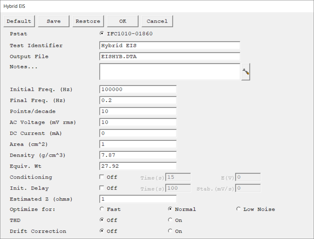
Test Identifier
A string that is used as a name. It is written to the data file, so it can be used to identify the data in database or data manipulation programs. The Identifier string defaults to a name derived from the technique's name. While this makes an acceptable curve label, it does not generate a unique descriptive label for a data set. The Identifier string is limited to 80 characters. It can include almost any normally printable character. Numbers, upper- and lower-case letters, and the most common punctuation characters including spaces are valid.
Output File
The name of the file in which the output data are written. By default, it is saved in the default file directory.
The input can be a simple file name with no path information. In this case the output file is located in the default file directory. The default file directory is specified in the Gamry.INI file under the [Framework] section with a Key named DataDir. The default path can be changed using the Path command in the Options menu. It can also include path information, such as C:\MY GAMRY DATA\YOURDATA.DTA. In this example, the data are written to the YOURDATA.DTA file in the MY GAMRY DATA directory on drive C. The default value of the Output File parameter is an abbreviation of the technique name with a *.DTA filename extension. We recommend that you use a *.DTA file name extension for your data file names. The data analysis package assumes that all data files have *.DTA extensions.
If the script is unable to open the file, an error message box, Unable to Open File, is generated. Common causes for this type of problem include:
•Invalid file name.
•The file is already open under a different Windows® application.
•The disk is full.
After you click the OK button in the error box, the script returns to the Setup where you can re-enter the file name.
Notes...
Enter several lines of text that describe the experiment. A typical use of Notes is to record the experimental conditions for a data set.
Notes defaults to an empty string and is limited to 400 characters. It can include all printable characters including numbers, upper- and lower-case letters, and the most common punctuation including spaces. Tab characters are not allowed in the Notes string. Press the Notes button on the right-hand side to open a separate Notes dialog box.
Initial Freq.
The starting frequency of the frequency sweep during data acquisition.
EIS scans are usually run with the Initial Freq. larger than the Final Freq. parameter. Refer to the potentiostat's Operator's Manual for detailed information on the applicable frequency range.
hertz (Hz)
Final Freq.
The final frequency of the frequency sweep during data acquisition.
The frequency sweep may not stop exactly at the final frequency. It is mathematically impossible to control both Points/decade and Final Freq. parameters exactly for all scan ranges. The EIS software chooses to control the Points/decade parameter exactly.
hertz (Hz)
Points/decade
The data density of the measured impedance spectrum. The data are spaced logarithmically and the number of data points in each frequency decade equals Points/decade. As a consequence, the frequency sweep may not stop exactly at the final frequency. It is guaranteed to do so only when the scan range contains an integer number of decades, such as 5 kHz to 0.05 Hz (five decades). You can use Initial Freq., Final Freq., and Points/decade to calculate the total number of data points in the spectrum.
Assuming that Initial Freq. = 5000 Hz, Final Freq. = 0.2 Hz, and Points/decade = 10:
The estimated number of points is always converted to an integer by truncating the fractional part of the number. The spectrum cannot contain more than 32000 data points. This is not a critical limitation because most impedance spectra contain fewer than 100 points.
AC Voltage
The amplitude of the desired AC Voltage signal which is measured at the cell. The applied current is changed to a value that should give the desired AC Voltage. Multiply the entered root-mean-square (rms) value by √2 (or ~1.414) to convert into a peak value.
Generally, you can enter AC Voltage values between 0.1 mV and 3000 mV. Values greater than 25 mV cause a non-linear response in most electrochemical systems and are therefore not recommended. The system does not control the AC Voltage exactly. It is satisfied with an AC Voltage close to the desired value. However, this inaccuracy does not carry over into the measured impedance, because an accurately measured AC Voltage is used in the impedance calculation.
mV rms
DC Current
The constant current applied to the cell throughout the frequency sweep. The AC Current is summed with the DC Current. In most cases, the DC Current should remain at its default value of zero. The discussion of the AC Voltage describes some limitations on the DC Current value.
mA
Area
The surface area of the sample that is exposed to the solution. The software uses the sample area to calculate the current density and corrosion rate (if applicable). If you do not want to enter an area, we recommend that you leaveit at the default value of 1.00 cm².
Do not enter a value of zero!
cm2
Density
The density of the metal sample, used in calculating the corrosion rate. You may disregard this parameter if absolute corrosion rates are not required for analysis.
g/cm3
Equiv. Wt
Theoretical mass of metal lost from the sample after one Faraday of anodic charge is passed. One Faraday of charge is equivalent to an Avogadro's number of electrons. The Equivalent Weight can be used to calculate the corrosion rate. You may disregard this parameter if absolute corrosion rates are not required.
To calculate the equivalent weight for an alloy, you need to know:
•The composition of the metal sample, expressed in mole fractions.
•The atomic weight AW of each alloy constituent.
•The number of electrons n, lost by each component of the sample as it oxidizes.
Suppose we have a 40:60 mole-percent Cu:Ni alloy dissolving in an acidic Cl–-solution. Ni forms Ni2+ as it dissolves and Cu forms a Cu+ complex. The equivalent weight is
The above discussion assumes that the sample oxidizes without changing the composition. This is not always the case. The de-zincification of brass is a well-known problem, where under special conditions brass becomes enriched in Cu as it corrodes. If selective dissolution occurs in your system, the best way to find the equivalent weight may be to measure the concentration of your corrosion products in the solution.
Conditioning
You may condition the electrode as the first step of the experiment, e.g., to remove an oxide film from the electrode or to grow one. Conditioning ensures that the metal sample has a known surface state at the start of the experiment. This step is done potentiostatically for a set amount of time.
Turn the conditioning phase On or Off with the Conditioning switch check box. Conditioning E is the potential applied during the conditioning phase of the experimental sequence. The conditioning potential has an allowed range of ±8 V. The resolution is 0.25 mV. If you have iR-compensation enabled for the data acquisition phase of your experiment, it is also turned on during conditioning. Conditioning E is always specified vs. Eref, because the open-circuit potential is not measured until after Conditioning is completed.
The Conditioning Time is the length of time that the sample is potentiostatted at Conditioning E. The minimum time is 1 s and the maximum time is 400000 s (more than 4 days). Below 1000 seconds, the time resolution is 1 s. Between 1000 and 10000 seconds, the resolution is 10 s, and 100 s above 10000 seconds.
seconds (s), volts (V)
Init. Delay
The Initial Delay phase of the experiment is the first step to occur in the experimental sequence. This phase of the experiment stabilizes the open-circuit potential of the sample prior to any applied signal and measures that open-circuit potential.
The Initial Delay is turned On or Off via the check box in the Setup dialog. The Initial Delay Time parameter is the time that the sample is held at the open-circuit potential prior to the scan. The delay may stop before the Initial Delay Time if the Stability criterion for Eoc is met. The minimum Delay Time time is 1 s and the maximum time is 400000 s (more than 4 days). Below 1000 seconds, the time resolution is 1 s. Between 1000 and 10000 seconds, the resolution is 10 s, and 100 s above 10000 seconds.
In many cases, you really do not want to set a delay for a fixed time, but you may want to a delay until Eoc stops drifting. The Stability parameter allows you to set a drift-rate that you feel represents a stable Eoc. If the absolute value of the drift-rate falls below the Stability parameter, the Initial Delay phase of the experiment ends immediately, disregarding the programmed Initial Delay Time. Enter a Stability setting of zero to ensure that the delay will last for the full Initial Delay Time. A typical value is 0.05 mV/s. The upper limit of this parameter is 8 V/s, well above the range of practical stabilities with real cells, while the lower limit is set by your patience. A stability of 0.01 mV/s indicates a drift of less than 1 mV within 100 seconds. The software will always take data long enough to resolve a 1 mV change in the potential at the requested drift rate.
No open-circuit voltage measurement occurs if the initial delay is turned off. In this case, the open-circuit voltage defaults to 0.0 V.
seconds (s), mV/s
Estimated Z
A user-entered estimate of the cell's impedance at the Initial Freq. parameter. It is used to limit the number of trials required before acquiring the first data point in an impedance spectrum. It is generally sufficient if Estimated Z is within a factor of five of the cell's impedance.
Before taking the first data point, the EIS software sets up the potentiostat and frequency response analyzer (FRA) to measure an impedance equal to Estimated Z and tries to measure the cell's impedance. If the estimate is fairly accurate, the first (or second) attempt to measure the impedance succeeds. If the estimate is poor, the system may take up to five trial readings before it finds the correct settings:
•After the first data point, the last measured impedance is used to calculate new measurement settings, so the entered Estimated Z becomes unimportant.
•An accurate Estimated Z is more valuable when the initial frequency is low. Remember, 1 mHz is 1000 s per cycle. Each impedance reading requires at least three cycles at a given frequency, so five readings to find a range at 1 mHz will take over 4 hours!
•There is no reason to enter values larger than 1 TΩ (1012Ω or smaller than 0.01 Ω, because these values drive the system settings to their most sensitive and least sensitive settings, respectively.After the first data point, the last measured impedance is used to calculate new measurement settings, so the entered Estimated Z becomes unimportant.
ohm
Optimize for
Select the sampling method for the experiment:
•Fast is the appropriate selection when the cell's stability is poor and a spectrum must be measured rapidly, or the system's impedance is low and well defined.
•Normal is the appropriate selection when the cell's impedance is high or the electrochemical system is noisy.
•The best data can be taken with Low Noise, but the time required to record an EIS spectrum can be quite long.
The EIS system tries to explain 99.9% of the variation in each Lissajous curve by fitting the E and I data to sine waves at the excitation frequency. It will record and average as many as 20 Lissajous curves to achieve this accuracy. There is a two-second delay after each data point to allow you to examine a Bode plot of the impedance spectrum.
With Fast, the time required to record a spectrum is much shorter (often by a factor of five). The fit accuracy is reduced from 99.9% to 99.5%. The maximum number of Lissajous curves is reduced, as low as two at low frequencies. The Lissajous curve is not displayed after the first ranging point, so there is no need for delays when the display changes.
THD
Enable Total Harmonic Distortion (THD) during the EIS experiment to obtain additional information about the system’s harmonics.
Drift Correction
Select On to enable Drift Correction. Both the original and the drift-corrected impedance values are separately calculated and recorded. The drift corrected impedance plot will be active by default but can be changed from the drop-down menu above the chart.
Drift Correction fits current and voltage data to a sine wave using a linear drift term, followed by non-linear least squares regression. Drift data are then subtracted from the current and voltage values and the corrected impedance Z is calculated via Fourier analysis.
Drift Correction is always disabled if an overload is detected, the frequency is above 10 Hz, or cycle decimation is occurring. Drift most commonly occurs at lower frequencies, which is why limitations are applied to this frequency range.