Description
Parameter |
Description |
Units |
||
|---|---|---|---|---|
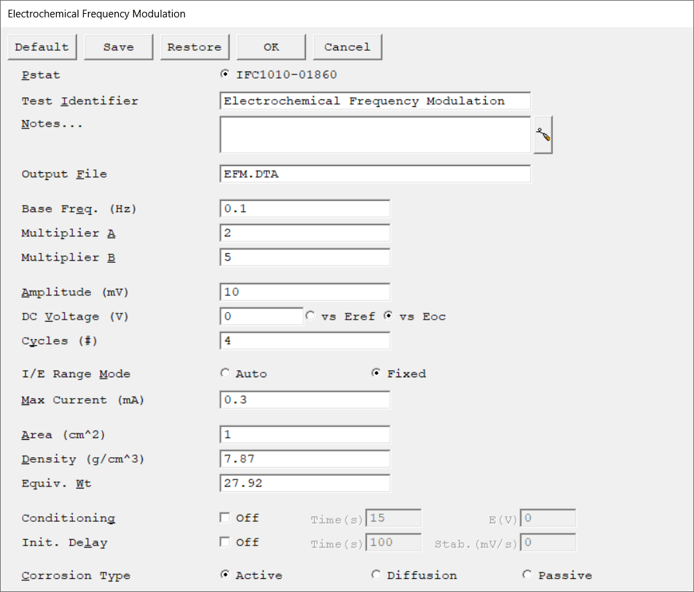
Select the potentiostat/galvanostat to perform the experiment. Each radio button corresponds to an installed potentiostat. You can select only one potentiostat at a time. Potentiostats that are already in use are marked with an asterisk. They can be selected but cannot be used. |
|
|||
A string that is used as a name. It is written to the data file, so it can be used to identify the data in database or data manipulation programs. The Identifier string defaults to a name derived from the technique's name. While this makes an acceptable curve label, it does not generate a unique descriptive label for a data set. The Identifier string is limited to 80 characters. It can include almost any normally printable character. Numbers, upper- and lower-case letters, and the most common punctuation characters including spaces are valid. |
|
|||
Enter several lines of text that describe the experiment. A typical use of Notes is to record the experimental conditions for a data set.
Notes defaults to an empty string and is limited to 400 characters. It can include all printable characters including numbers, upper- and lower-case letters, and the most common punctuation including spaces. Tab characters are not allowed in the Notes string. Press the Notes button on the right-hand side to open a separate Notes dialog box. |
|
|||
The name of the file in which the output data are written. By default, it is saved in the default file directory.
|
|
|||
The repeat time of the EFM waveform applied to the cell. The two frequencies simultaneously applied to the cell are:
|
hertz (Hz) |
|||
Multiplier A and Multiplier B define the EFM waveform applied to the cell. The two frequencies simultaneously applied to the cell are:
|
|
|||
|
||||
The amplitude of each of the two sine waves. Keep in mind that the total EFM waveform amplitude typically ranges between 1 and 2 times of the selected value due to the principle of superposition.
Choose an amplitude that is small compared to the Tafel constants but large enough to give a reasonable signal. For many systems, 10 to 40 mV is a good starting point. |
mV |
|||
The constant potential applied to the cell throughout the EFM scan. For most EFM experiments, the DC Voltage is 0 V versus the open-circuit potential |
volts (V) |
|||
The number of times the scan is repeated during the experiment.
The Number of Cycles and the Base Frequency determine the duration of an EFM experiment. The greater the cycle number, the longer the experiment takes, but the resolution between the peaks of the intermodulation spectrum increases. Although you may enter any number of cycles, you get better results if Number of Cycles has a power of two: 2, 4, 8, ... 128, with a maximum number of 255. The first repetition of the Base Frequency (the first cycle) is not used for data analysis. The duration of an EFM experiment can be calculated as follows:
|
|
|||
Select the current range mode and choose between Auto mode or Fixed mode.
Because the EFM waveform is a complicated AC waveform, better results are generally obtained in the Fixed mode. In Fixed mode, the current scale is selected based on Max Current. In Auto mode, Max Current is used as an initial guess for the proper scale, but subsequent decisions are based on the value of the most recently measured current. |
|
|||
Max Current controls the current measurement range if I/E Range is set to Fixed mode. If I/E Range is set to Auto mode, Max Current specifies the maximum expected starting current.
The software adjusts the current range based on the Max Current input. In order to use the most sensitive range that will not overload, the software chooses the current range based on a value that is 89% of the full-scale current range.
|
mA |
|||
The surface area of the sample that is exposed to the solution. The software uses the sample area to calculate the current density and corrosion rate (if applicable). If you do not want to enter an area, we recommend that you leave it at the default value of 1.00 cm².
|
cm2 |
|||
The density of the metal sample, used in calculating the corrosion rate. You may disregard this parameter if absolute corrosion rates are not required for analysis. |
g/cm3 |
|||
Theoretical mass of metal lost from the sample after one Faraday of anodic charge is passed. One Faraday of charge is equivalent to an Avogadro's number of electrons. The Equivalent Weight can be used to calculate the corrosion rate. You may disregard this parameter if absolute corrosion rates are not required.
To calculate the equivalent weight for an alloy, you need to know: •The composition of the metal sample, expressed in mole fractions. •The atomic weight AW of each alloy constituent. •The number of electrons n, lost by each component of the sample as it oxidizes.
|
g/equivalent |
|||
You may condition the electrode as the first step of the experiment, e.g., to remove an oxide film from the electrode or to grow one. Conditioning ensures that the metal sample has a known surface state at the start of the experiment. This step is done potentiostatically for a set amount of time.
|
seconds (s), volts (V) |
|||
The Initial Delay phase of the experiment is the first step to occur in the experimental sequence. This phase of the experiment stabilizes the open-circuit potential of the sample prior to any applied signal and measures that open-circuit potential.
|
seconds (s), mV/s |
|||
The calculation of the corrosion current from EFM data depends on the mechanism of the corrosion process. The three choices are Active, Diffusion control, and Passive film control. The choice here only determines the equation for the run-time display. You may change your choice later in the Echem Analyst 2™ and recalculate the corrosion rate without having to rerun the experiment. |
|

