Description
Parameter |
Description |
Units |
||
|---|---|---|---|---|
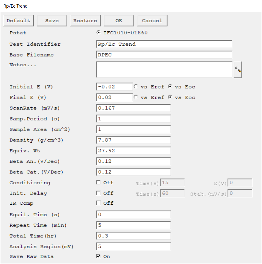
Select the potentiostat/galvanostat to perform the experiment. Each radio button corresponds to an installed potentiostat. You can select only one potentiostat at a time. Potentiostats that are already in use are marked with an asterisk. They can be selected but cannot be used. |
|
|||
A string that is used as a name. It is written to the data file, so it can be used to identify the data in database or data manipulation programs. The Identifier string defaults to a name derived from the technique's name. While this makes an acceptable curve label, it does not generate a unique descriptive label for a data set. The Identifier string is limited to 80 characters. It can include almost any normally printable character. Numbers, upper- and lower-case letters, and the most common punctuation characters including spaces are valid. |
|
|||
The name of the file in which the output data are written. By default, it is saved in the default file directory.
|
|
|||
Enter several lines of text that describe the experiment. A typical use of Notes is to record the experimental conditions for a data set.
Notes defaults to an empty string and is limited to 400 characters. It can include all printable characters including numbers, upper- and lower-case letters, and the most common punctuation including spaces. Tab characters are not allowed in the Notes string. Press the Notes button on the right-hand side to open a separate Notes dialog box. |
|
|||
The starting potential of the potential sweep during data acquisition. The allowed range is ±10 V with a resolution of 0.125 mV. Its accuracy is determined by the settings of Initial E and Final E. |
volts (V) |
|||
The final potential of the potential sweep during data acquisition. The allowed range is ±10 V with a resolution of 0.125 mV. Its accuracy is determined by the settings for Initial E and Final E. |
volts (V) |
|||
The speed of the potential sweep during data acquisition.
|
mV/s |
|||
The spacing between data points. The minimum value that we recommend is 0.1 s. The longest Sample Period allowed is 600 s.
|
seconds (s) |
|||
The surface area of the sample that is exposed to the solution. The software uses the sample area to calculate the current density and corrosion rate (if applicable). If you do not want to enter an area, we recommend that you leave it at the default value of 1.00 cm².
|
cm2 |
|||
The density of the metal sample, used in calculating the corrosion rate. You may disregard this parameter if absolute corrosion rates are not required for analysis. |
g/cm3 |
|||
Theoretical mass of metal lost from the sample after one Faraday of anodic charge is passed. One Faraday of charge is equivalent to an Avogadro's number of electrons. The Equivalent Weight can be used to calculate the corrosion rate. You may disregard this parameter if absolute corrosion rates are not required.
To calculate the equivalent weight for an alloy, you need to know: •The composition of the metal sample, expressed in mole fractions. •The atomic weight AW of each alloy constituent. •The number of electrons n, lost by each component of the sample as it oxidizes.
|
g/equivalent |
|||
Anodic β (Tafel) coefficient used to calculate the corrosion current Icorr. The value can be adjusted later within the analysis software. |
volts/decade |
|||
Cathodic β (Tafel) coefficient used to calculate the corrosion current Icorr. The value can be adjusted later within the analysis software. |
volts/decade |
|||
You may condition the electrode as the first step of the experiment, e.g., to remove an oxide film from the electrode or to grow one. Conditioning ensures that the metal sample has a known surface state at the start of the experiment. This step is done potentiostatically for a set amount of time.
|
seconds (s), volts (V) |
|||
Use the Initial Delay parameter to tell the system your definition of a stable potential and when to begin the actual measurement. If the absolute value of the Eoc drift-rate falls below the Stability parameter, the Initial Delay phase ends immediately and the experiment begins, disregarding the Time parameter. The drift rate can never fall below zero, so entering a Stability value of zero ensures that the Initial Delay will not end prematurely. A typical value is 0.05 mV/s. The lower limit of the Stability parameter is set by your patience. For example, a stability of 0.01 mV/s indicates a drift of less than 1 mV within 100 seconds. |
seconds (s), mV/s |
|||
Choose to turn iR-compensation either On or Off. Turning on IR Comp causes the applied potential to be adjusted for the estimated iR-drop.
Gamry potentiostats are able to estimate uncompensated voltage-drop caused by cell resistance. They do so by performing a current-interrupt experiment after every data point. |
|
|||
The duration during which the cell remains at the initial potential, with the cell turned on before data acquisition begins. It allows the system to equilibrate before the actual experiment starts. No data are recorded during this step.
|
seconds (s) |
|||
The time (specified as hours:minutes) between each test on the cell. For example, if the first test begins at 2:08 and the Repeat Time is 30 minutes, additional tests occur at 2:38, 3:08, 3:38, etc. |
minutes (min) |
|||
The duration of the experimental run. The script keeps track of the elapsed time from the start of the experiment. At the start of each test, the elapsed time is compared to the Total Time. If the elapsed time is greater than or equal to the Total Time, the experiment is halted and the Runner window is closed.
The Total Time is always entered in hours. Fractional hours can be entered as decimal numbers. To run a single test, enter a Total Time equal to the Repeat Time or simply run the Polarization Resistance experiment. For N tests, enter a Total Time = N × Repeat Time.
|
hours (hr) |
|||
The region over which the linear fit is performed on the data. It is bounded by x mV positive and negative from the open-circuit potential. For example, if the sample has an open-circuit potential of 0 V and the Analysis Region is 5 mV, the linear fit is performed on data from –5 mV to +5 mV. |
mV |
|||
If enabled, individual Polarization Resistance data files are recorded and saved in addition to the Rp/Ec Trend data file.
The file names of the raw data files consist of the main file's name, followed by an underscore and the repeat number in which the data was recorded.
|
|

